UNIT 3: ADTs and LSQs
Table of Contents
1 Abstract Data Types
Allegedly, this course is about Data Structures. In actuality, it is about Abstract Data Types (ADTs) and their implementation with Data Structures. An ADT is a description of an interface, and the data structures are how we make them work. For instance, last semester, we built a Queue. A Queue is an ADT; the linked list is the data structure.
1.1 The List ADT
We've been using the List ADT in our homework assignments, and so
far you've seen two different implementations of a List: the
FixedList and the recursive LinkedList. To review, here are the
following methods that must be defined for a List
get(i): return the data at thei-th place in the list.<set(i,e): return thei-th piece of data, and also replace it with e.add(i,e): insertein the list at locationi. All data with locations greater thaniare shifted to a location one greater.remove(i): remove and return the data ati. Shift all data at higher indices down.size()return the number of elements in the list.
This is all an ADT is! Any way of making this work, no matter how
stupid or slow, still means that it is an it is a list. However,
implementing it with different data structures gives us different run
times, and thus the choice of implementation can have a big impact on
the performance of your program. Perhaps you should use an array back
end, like FixedList or ArrayList, or a linked node structure like
LinkedList. Presumably, you could implement all four of
those methods with a combination of strategies.
1.2 Generic Storage
Another important thing to consider with ADT's is that they do not
specify what kind (or type) of element they can store. Looking at the
definition above and in the code samples provided in the first few
homework, the type of e is undefined, just referred to as an
element. This generalization of the ADT is called generics in Java,
and templates in C++. And, most Object Oriented programming
languages have a notion of generalizing data structures.
As an example of generics, consider defining a LinkedList implementation
of Strings, which may have the following Java decelerations:
public class LinkedList implements List{

    private class Node{
        String data;
        Node next;
    }

    Node head = null;

    void set(int i, String e){/*---*/}
    String get(int i){/*---*/}
    void add(int i, String e){/*---*/}
    String remove(int i){/*---*/}
    int size(){/*---*/}
}
This implementation is fine and well whenever we want to store
String's, but what if we want to store int's or double's or
Object's or whatever we want? We have to copy paste the code and
create a whole new implementation at each of the types. That, is
simply, a nightmare for a programmer.
What we want is to write one implementation of the data structure
that can store all the things we want. One way to do this is to
leverage the subclassing in Java and recognize that Object is the
base type, and, thus, everything is a subclass of Object. Maybe we
could define our LinkedList implementation like so:
public class LinkedList implements List{

    private class Node{
        Object data; //<---
        Node next;
    }

    Node head = null;

    //rest of methods to follow ...
    void set(int i, Object e){/*---*/}
    Object get(int i){/*---*/}
    void add(int i, Object e){/*---*/}
    Object remove(int i){/*---*/}
    int size(){/*---*/}
}
Now when we use this implementation, we have to cast the elements going in and going out of the data structure as the implementation expects and returns Objects, not the specific type we are using. For example:
List l = new LinkedList();

l.add(0, (Object) "Go"); //Cast to object
l.add(1, (Object) "Navy");

//Cast to String
System.out.println("" + ((String) l.get(0)) + ((String) l.get(1)));
While this is better, you should feel dissatisfied. Foremost, all that casting is a runtime check, meaning that if you make a mistake it won't be noticed until you actually run the program. That may be too late to actually fix the mistake. What we would prefer is for Java to be able to recognize what type the list is suppose to store and ensure that all our use cases match that type.
That is exactly what generics do. You define the type for the class in
greater-then and less-then brackets, and this acts as a
"meta-argument" to the constructor defining the type that is being
stored. Using generics, we get the definition of the LinkedList from
the homework:
public class LinkedList<T> implements List<T>{

    private class Node{
        T data;
        Node next;
    }

    Node head = null;

    //rest of methods to follow ...
    void set(int i, T e){/*---*/}
    T get(int i){/*---*/}
    void add(int i, T e){/*---*/}
    T remove(int i){/*---*/}
    int size(){/*---*/}
}
Notice that we've specified a new type-variable, T, that defines
what type of elements the LinkedList stores.
1.3 Iterators and Lists
To motivate iterators, consider the following simple code for
iterating over a List l.
for(int i=0;i<l.size();i++){
    l.get(i);
}
What is the runtime of this procedure? First consider the ArrayList
or FixedList implementation which uses an underlying array
storage. It's, \(O(n)\), right? The get() operation requires a
constant number of operations to access the array at index i and
return the element.
What if we are using the recursive LinkedList implementation? To
get() an element we must traverse from the head of the list to index
i. If we do that \(n\) times, we are left with the following summation
and calculation (see this article for calculating the sum of the
natural numbers).
Frankly, that sucks. This should clearly be \(O(n)\). How do we get there?
The problem with the iteration above for linked list is that it
doesn't preserve any state when you are doing the iteration. Every
get() requires you to start over! That's where the additional \(n\)
factor comes in and you get \(O(n^2)\) instead of \(O(n)\).
Java provides a means to overcome this issue using an Iterator, and
you can find the documentation here. The Iterators interface defines
three methods (where E is the generic):
//return true if the iteration has more elements
boolean hasNext();

//Returns the next element in the iteration
E next();

//Removes from the underlying collection the last element returned by
//this iterator (optional operation)
void remove();
What this interface enables is that a new Iterator is generate at
the start of each iteraction, storing where in the iteration we are
at. You can keep call next() until there is no more elements, and
you can check the case where we've reached the end using
hasNext(). The remove() interface is optional.
We won't spend too much time implementing Iterator's in this class,
but just to show you how this all fits together, here's an Iterator
implementation for the recursive LinkedList:
import java.lang.Iterable;
import java.lang.Iterator;

//now implements Iterable
public class LinkedList<T> implements List<T>,Iterable<T>{

    private class Node{
        T data;
        Node next;
    }

    Node head = null;

    //rest of methods to follow ...
    void set(int i, T e){/*---*/}
    T get(int i){/*---*/}
    void add(int i, T e){/*---*/}
    T remove(int i){/*---*/}
    int size(){/*---*/}

    //Iterable interfaces require that you can return an Iterator
    public Iterator<T> iterator(){
        return new LLIteartor<T>(head);
    }

    //the Iterator we will return
    private class LLIterator implements Iterator<T>{
        private Node cur;

        public LLIterator(Node start){cur=start;}

        public boolean hasNext(){ return cur!=null; }

        public T next(){
            T data = cur.data;
            cur = cur.next;
            return data;
        }

        public void remove() { throw new UnsupportedOperationException();}
    }

}
Now, we can use the LinkedList in a foreach iteration like so:
LinkedList<String> l = new LinkedList<String>();
l.add(0,"Go Navy!");
l.add(1,"Beat Army!");

//foreach iteration, assign s to each element in l using the Iterator methods
for(String s : l){
    System.out.println(s); //prints "Go Navy!\nBeat Army!\n"
}
1.4 The size() method for List
You can pretty easily imagine how size() is implemented for an
array-based list — you just get the length of the array. But for a
linked list, we have been iterating over the whole list and counting,
taking \(O(n)\), right?
Well, all that work could be easily avoided by storing one extra
little piece of data in the Linked List class; namely, an int for
the current size of the list. This value would be updated on each
add() or remove() operation, and returned by each a call to
size().
public class LinkedList<T> implements List<T>,Iterable<T>{

    private class Node{
        T data;
        Node next;
    }

    Node head = null;
    int length = 0;

    //rest of methods to follow ...
    void set(int i, T e){/*---*/}
    T get(int i){/*---*/}
    void add(int i, T e){/*---*/}
    T remove(int i){/*---*/}

    int size(){ return length;}
There is something subtle but important about why this is okay: An ADT implementation is allowed to store extra data besides whatever information the ADT itself specifies.
In the case of a List, the ADT just specifies that you are storing an ordered sequence of elements. It says nothing about storing the size. But your data structure is allowed to store the size, in order to make the <code>size()</code> operation more efficient! The key is actually that the total storage is still the same in terms of big-O, since \(n+1 \in O(n)\).
2 Amortizing The Cost of ArrayLists Expansion
Given the previous table, it is hard to remember where the advantages of Linked Lists comes from, but they are advantages. Particularly, Linked Lists are much better when adding to the ends of the list, either the front or the back because it only requires reassigning the pointers.
With linked lists, regardless if you are inserting at the front or the end, this is \(O(1)\). Array Lists, however, are \(O(n)\).
This fact may not be obvious at first, but consider that if you were to insert at the beginning of the list, which corresponds to index 0 in the underlying storage array, to make space for that element requires shifting the other \(n\) elements to the right. That's \(O(n)\).
You might think that inserting at the end of the list would improve things, and, if there is space in the storage array, that operation will be constant time. But, that doesn't tell the whole story and is the best case scenario. What about the worst case scenario? What if the storage array is full?
If the storage array is full, then you've got to make more space. The only way to do that is to create a new and larger array and then copy all the elements into the new array, including the new value to add. The copying of all the elements, that's \(O(n)\).
So, in both special cases, inserting at the front or back of an Array List is going to be \(O(n)\), so it would seem, if you are in such circumstances, the Linked List reigns supreme. However, this doesn't paint the full picture. It is possible to make adding to the end of an array-based list significantly faster.
2.1 Doubling Array Storage on Expansion
Let's use the scheme that every time we run out of room on our array, we double the size of the array. Will we have lots of unused indices? Yup. But, if our biggest number of elements in the list is \(n\), the most memory we'll use is \(2n\). And, while that might hurt, at least that's still \(O(n)\). (Yup! We can (and do) use Big-O in reference to memory, too!)
Now, we only resize every time we actually fill this too-big array. Isn't the worst case still O(n)? Well, sort of. For the first time, our "number of operations as a function of \(n\)" function isn't smoothly increasing; instead, it's spiky. This is because almost all of the time, adding to the end is O(1) because there will be space for the new element. However, every now and then, it's O(n). See:
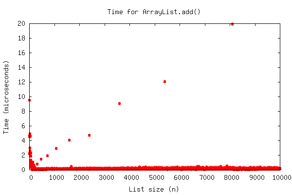
If you drew a line threw those little red "outlier" dots, it'd be a straight line; \(O(n)\). But almost all the dots are right there at the bottom, \(O(1)\), not increasing at all even with thousands of elements in the array.
What we'd like to say is that those \(O(n)\) dots don't ultimately matter, and the real cost is \(O(1)\). Amortized analysis is what lets us say this and still be mathematically correct.
2.2 Amortized Analysis
Pretend you have a business. Every 10 years, you have to buy a $100,000 machine. You have two ways you could consider this; either, every ten years you lose massively, having to pay $100,000, or every year you put aside $10,000 to be used later. This is called amortizing the cost. We can do the same thing here.
Let's assume assigning one element to an array is 1 operation. Again, if we
double the size of the array every time we need more space, starting with an
array of size one, we would get the following series of costs when adding 17
elements to an initially-empty array: 1 2 3 1 5 1 1 1 9 1 1 1 1 1 1 1 17.
The reason is that when the size reaches \(1, 2, 3, 5, 9, 17\), which is 1 more than each power of 2, we have to allocate a new array and copy everything over. So those are the "outlier" and expensive additions. But all the other additions are cheap; they just involve copying a single element.
But we can amortize these expensive additions over the previous "cheap" ones! Check it out:
| Size | 1 |
2 |
3 |
5 |
9 |
17 |
| Actual | 1 |
1 2 |
1 2 3 |
1 2 3 1 5 |
1 2 3 1 5 1 1 1 9 |
1 2 3 1 5 1 1 1 9 1 1 1 1 1 1 1 17 |
| Amortize | 1 |
3 0 |
3 3 0 |
3 3 3 3 0 |
3 3 3 3 3 3 3 3 0 |
3 3 3 3 3 3 3 3 3 3 3 3 3 3 3 3 0 |
Noticing the theme? No matter how big our list becomes, the amortized cost of a single add never gets bigger than 3. So, the cost of an add, even with resizing the array, is \(O(1)\) (amortized).
Another way of putting this is that the sum total cost of a series of \(n\) additions onto the end of an initially-empty array is \(O(n)\). In fact, if we take the same graph as above and plot the running sum instead of the individual cost of each operation, the fact that this line is \(O(n)\) becomes fairly obvious:
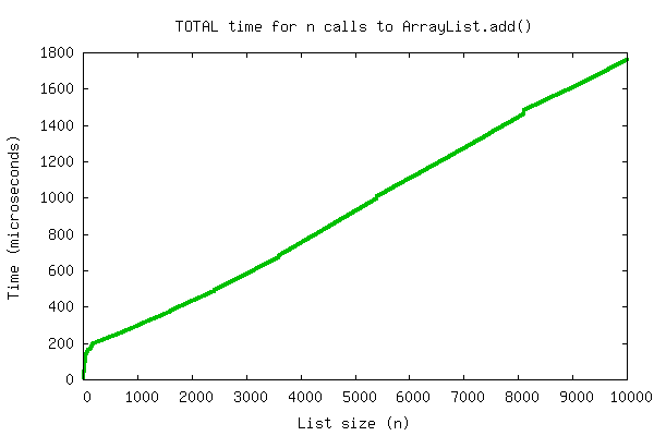
As you may already know, this is in fact exactly how Java's ArrayList
class works. Using similar ideas they can also remove from the end of an
ArrayList in \(O(1)\) amortized time, and guarantee that the space usage is
kept at \(O(n)\). In fact, the previous graphs came from timing Java's own
ArrayList!
There is one additional problem with the doubling-size array implementation
of a List: the size of the array no longer matches the size of the list! So
just like with linked lists, we have to store an extra int for the
"actual" size of the list, which will always be less than the size of the array.
Again, this keeps the storage as \(O(n)\) and so it's okay.
2.3 What if we don't double the size of the array on expansion?
It is very important for amortized analysis that the storage array doubles when it is full, otherwise the analysis from before falls apart. The add-to-back operation becomes \(O(n)\) again. To see this we must use a bit of notation to express the amortized concepts from above. First, lets show, again, that the amortized cost of add-to-back for an array list that expands by doubling is \(O(1)\). Using that baseline, we can show that if we do something less than doubling, say constant size expansion, we go back to being an \(O(n)\) operation.
2.3.1 Showing that add-to-back is O(1) amortized for doubling
Let's do the analysis of doubling the array on expansion, but this time with a bit more math. To start, we can define a term \(c_i\) that is the cost of the i-th insertion to the end of the list. This would be the formula for the "Actual" row in the table from above (where a non-expanding insert only costs one step).
\[ c_i = \begin{cases} i & \text{if } \ \ (i-1) \ \ \text{is a power of 2}\\ 1 & otherwise\\ \end{cases} \]
In the above definition, it costs either constant time, 1 step, or i steps to do the insertion. It costs i steps when (i-1) is a power of 2, which is when we do expansions. What we must now show to demonstrate \(O(1)\) amortized cost is that total costs of \(n\) insertions should be \(O(n)\) for add-to-back insertion, and thus each individual insertion costs \(O(1)\) amortized. That's the same argument we made above, and mathematically we can write the summation.
\[ \sum_{i=1}^{n} c_i = n-\lfloor lg(n) \rfloor + \sum_{j=0}^{ \lfloor lg(n) \rfloor } (2^j + 1) \]
Solving the summation we recognize that there is \(n - \lfloor lg(n) \rfloor\) operations that cost a constant amount of time, where we are subtracting the number of times we need to expand the array, \(\lfloor lg(n) \rfloor = \lfloor log_2(n) \rfloor\). The next item to solve for is the cost of all the expansions. Since we expand on powers of 2 and do we do so \(\lfloor lg(n) \rfloor\) times, the cost of the number of expansions is solving the following summation.
\begin{array}1 \sum_{j=0}^{ \lfloor lg(n) \rfloor } 2^j + 1 &= \sum_{j=0}^{ \lfloor lg(n) \rfloor } 2^j + \sum_{j=0}^{ \lfloor lg(n) \rfloor } 1\\ &= \sum_{j=0}^{ \lfloor lg(n) \rfloor } 2^j + \lfloor lg(n) \rfloor &= 2n - 1 + \lfloor lg(n) \rfloor \end{array}Fortunately, the solution involves the geometric sum, whose solution is as follows.
\[ \sum_{i=0}^{n-1} r^i = \frac{1-r^n}{1-r} \]
Substituting in 2 for \(r\), we get that \(\sum_{j=0}^{ \lfloor lg(n) \rfloor } 2^j = 2n-1\). And, we now have everything to complete the analysis.
\[ \sum_{i=1}^{n} c_i = n-\lfloor lg(n) \rfloor + 2n - 1 + \lfloor lg(n) \rfloor = 3n - 1 \]
This says it costs \(O(n)\) to insert \(n\) items to the end of the list, thus each insertion costs \(O(1)\) amortized.
2.3.2 Showing that add-to-back is O(n) amortized with constant size expansion
Let's do the same analysis again, but this time instead of doubling the list, we expand by a constant factor. For example, we start with a list of size \(k\) and once the array is full, we will expand it to size \(2k\), and then to \(3k\), and so on. In that scenario, we define \(c_i\), the cost of each insert like so:
\[ c_i = \begin{cases} i & \text{if } \ \ (i-1) \ \text{ mod } \ k = 0\\ 1 & otherwise\\ \end{cases} \]
The cost of insert is O(n) at each factor of \(k\) because that is when the array is full and must be copied into a new array. If we consider the costs of \(n\) insertions to the end of the list, we can again solve the summation, but it looks a bit different now.
\[ \sum_{i=1}^{n} c_i = n - \lfloor n/k \rfloor + \sum_{j=0}^{\lfloor n/k \rfloor} k \cdot j \]
From this summation, it is clear that there are many constant operations, but there are now many more non-constant operations \(\lfloor n/k \rfloor > \lfloor lg(n) \rfloor\) as expansion occurs on each factor of \(k\) rather than each power of 2. Further, looking at the costs of the expansions, for the total number of times we expand, it costs \(k \cdot j\) where \(j\) is the count of the number of expansion. We know how to solve the sum for the cost of all the summation as it is just a sum of a sequence of numbers:
\[ \sum_{j=0}^{\lfloor n/k \rfloor} k \cdot j = k \cdot \sum_{j=0}^{\lfloor n/k \rfloor} j = k \cdot \left ( \frac{\lfloor n/k \rfloor (\lfloor n/k \rfloor + 1)}{2} \right) = \frac{k}{2}({\lfloor n/k \rfloor}^2 + \lfloor n/k \rfloor) \]
Substituting that back into the other formula, we get this result for the cost of \(n\) insertions.
\[ \sum_{i=1}^{n} c_i = n - \lfloor n/k \rfloor + \frac{k}{2}({\lfloor n/k \rfloor}^2 + \lfloor n/k \rfloor) \]
If you look closely, you see the \({\lfloor n/k \rfloor}^2\) term dominates, which makes this \(O(n^2\)) to insert \(n\) items to the end of the list with constant expansion. Thus it is \(O(n)\) amortized to insert each item, and that is no good.
Finally, you can also see this fact clearly if were to measure the speed of two routines, one using doubling expansion and one using constant expansion.
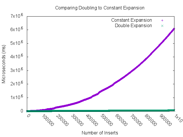
Cearly, the constant expansion is increasing faster than the doubling expanding line, and precisely, one is \(O(n^2)\) and the other \(O(n)\). The moral of the story is that you have to (at least) double the size of the array when expanding otherwise you do not get \(O(1)\) amortized costs of expansion.
3 Stacks
3.1 Stacks ADT
Our second ADT is the Stack. We're pretty familiar with Stacks already, so this might not be so hard. Stacks work like a stack of plates: you only add plates onto the top of the stack, and you only remove stacks from the top of the stack. This makes them a LIFO (last-in-first-out).
The methods of a stack are:
push(e): Add element e to the top of the stack.pop():Take the top element off the top of the stack, and return it.peek(): Return the top element of the stack, without altering the stack.size(): Return the number of elements in the stack
Let's consider an example. On the left column of this table, I will have some commands. In the middle, I'll put what is returned, if anything. On the right, I'll put the state of the stack, with the top of the stack on the left.
| Command | Returend Value | Stack |
|---|---|---|
| empty | ||
push(3) |
- | 3 |
push(5) |
- | 5 3 |
pop() |
5 |
3 |
peek() |
3 |
3 |
push(4) |
- | 4 3 |
peek() |
4 |
4 3 |
pop() |
4 |
3 |
pop() |
3 |
empty |
3.2 Stack Implementations
Implementation with Linked Lists should seem relatively easy to you;
if "first" refers to the top element of the stack, then push() is
just an add-to-front, pop() is a remove-from-front, and peek is just
return first.getData(); (modulo error checking for an empty
stack, of course).
This means that for stacks implemented by linked lists, all three methods can be run in \(O(1)\) time. Great!
What about arrays? Well, if we used a "dumb" array, each push() and
pop() would cost \(O(n)\) because of the need to copy the entire
contents each time. But as we saw above with amortized ArrayList, we
can be smart about this and leave some empty space in the array,
doubling it when necessary. You could technically also shrink the
array (halving when necessary) in pop(), but that makes everything
more cumbersome, so we'll assume the resizings only happen during
push() only.
| LinkedList | ArrayList | |
|---|---|---|
push() |
\(O(1)\) | \(O(1)\) amortized |
pop() |
\(O(1)\) | \(O(1)\) |
peek() |
\(O(1)\) | \(O(1)\) |
3.3 Usefulness of Stacksh
OK, so stacks are fast! What can we do with them?
- Reverse stuff - pushing everything on, and then popping it all off puts it in reverse order.
- Maze solving - every time you come to a junction, push it on the stack. When your decision doesn't work out, pop to the last junction, and go the other way. If there are no more possible directions, pop again.
- For more complex uses of stacks, stay tuned…
And, you'll see Maze solving in the project!
4 Queues
4.1 Queue ADT
We know Queues well from IC211. If a Stack is a LIFO (Last-In First-Out), then a Queue is a FIFO (First-In First-Out). In other words, things come out in exactly the same order they went in.
Think about a line for the checkout counter at the grocery store (after all, "queue" is British for "line"). People can only join the line at the end, and only leave the line at the front. In between, they never switch order.
The methods a Queue must have are:
enqueue(e): Add an element to the back of the Queuedequeue(): Remove and return the front element of the Queuepeek(): Return, but do not remove, the front element of the Queuesize(): Return the number of elements in the queue
4.2 Implementing a Queue with a Linked List
Implementation with a Linked List is fairly straightforward. Enqueue
is just an add-to-back operation, which is \(O(1)\) if we have a tail
reference to track the last Node in the linked list. Just like we
discussed with the size() operation, adding new book keeping
elements is totally fine for a ADT.
Dequeue is also simple, and is remove-from-front operation, which,
again, is \(O(1)\). We already track the front of the list with a head
reference, so we are good to go there.
Finally, peek() is the same as dequeue() but without removal. That
operation just returns the value of the first Node in the list, like
head.getData(), which is clearly \(O(1)\).
So, Linked Lists are great(!) at implementing Queues. What about ArrayLists?
4.3 Implementing a Queue with Array Storage
4.3.1 Challenges of using an ArrayList for Queues
The challenge of using array storage to implement a Queue is hindered by have to tracking the first element in the queue. There are two obvious choices for this, the front of the queue could either be index 0 or the list or the size-1 of the list (or the last element in the list).
If we were to use index 0 as the head of the queue, then enque is simply an add-to-back operation which we know is \(O(1)\) amortized. But what about dequeue? When we dequeue an element, we are performing a remove-from-front operation, and that requires shifting the remaining elements towards the front. For a naive array implementation, that could be \(O(n)\), and that's bad.
We come up against a similar problem if we were to use size-1 as the front of the queue. In that case dequeue is \(O(1)\) since you are removing from the end of the list, but enqueue is now an add-to-front operation, which requires shifting all the elements to the right in the storage array. The shifting operation is \(O(n)\).
So, it would seem that ArrayLists simply are no good for implementing queues. That's true, but we can make some small changes and get back constant time operations.
4.3.2 Circular Array Lists
One way to solve this is with a modified ArrayList called a
CircularArrayList. In the circular version, you track the number of
elements in the list (length) and the current first index
(head). For example:
public class CircularArrayList<T> implements List <T>{

 private int head=0;
 private T elements[];

 //..
}
The difference between an ArrayList and a CircularArrayList is
that the start index of an ArrayList doesn't change, but it may in a
CircularArrayList. And, in particular, the head of the
CircularArrayList changes in a remove-from-front operation.
  |
  v
.---------------------------.     size()=4
| 0 | 1 | 2 | 3 |   |   |   |     head=0
'---------------------------'

remove(0) or dequeu()

      |
      v
.---------------------------.     size()=3
|   | 1 | 2 | 3 |   |   |   |     head=1
'---------------------------'

remove(0) or dequeu()

          |
          v
.---------------------------.     size()=2
|   |   | 2 | 3 |   |   |   |     head=2
'---------------------------'
Enqueue, or the add-to-back operation, becomes a bit more complicated
because we need to calculate the end of the list. It is no longer just
at array[length] as it was in the ArrayList implementation. But,
it's easy to calculate as array[head+length], and we can perform any
add()'s there and continue to well track the list.
add(size(),4); or enqueue(4)

          |
          v
.---------------------------.     size()=3
|   |   | 2 | 3 | 4 |   |   |     head=2
'---------------------------'


add(size(),5) or enqueue(5)

          |
          v
.---------------------------.     size()=4
|   |   | 2 | 3 | 4 | 5 |   |     head=2
'---------------------------'

add(size(),6) or enqueue(6)

          |
          v
.---------------------------.     size()=5
|   |   | 2 | 3 | 4 | 5 | 6 |     head=2
'---------------------------'
The next issue we need to consider is, what happens when we've reached
the end of the array? Well, there may be more free slots in the front
of the array if the head > 0. What we want to do is wrap-around,
and it's easy to do that calculation using a modulo to determine the
end of the list array[(head+size())%array.length] (or any requested
index in the list, where head is replaced by i, the index being
requested).
In the end, after one more enque() / add() in the example above, we
have the following array layout.
add(size(),7) or enqueu(7)

          |
          v
.---------------------------.     size()=6
| 7 |   | 2 | 3 | 4 | 5 | 6 |     head=2
'---------------------------'
This wrapping around is why we call it a circular array list because, over time with adds and removes, the front and end of the list circle back around on each other.
The last implementation detail to consider is the resizing: What
happens when the array is completely full? Fortunately, this is the
same as expanding the storage array for an ArrayList, and we know
that this cost can be amortized over all the add() operations. (If
you want to, when you resize, you could even rearrange the array such that
head becomes 0 again).
Now, it should be clear to you that an add-to-front and and a
remove-from-back for a CircularArrayList is \(O(1)\) amortized and
\(O(1)\), respectively.
| LinkedList | ArrayList | CircularArrayList | |
|---|---|---|---|
enqueue() |
\(O(1)\) | \(O(1)\) amortized | \(O(1)\) amortized |
dequeue() |
\(O(1)\) | \(O(n)\) | \(O(1)\) |
peek() |
\(O(1)\) | \(O(1)\) | \(O(1)\) |
Credit: Ric Crabbe, Gavin Taylor and Dan Roche for the original versions of these notes.