UNIT 1: Big-O Notation
Table of Contents
1 Big-O Notation
1.1 What is a Data Structure
Most of you carry around (the same) large black backpack all day. Think about what's in there, and where it is. Your decisions on what to put in there and where to put it all were governed by a few tradeoffs. Are commonly-used things easy to reach? Is the backpack small and easy to carry? Is it easy to find everything in there? Do you really need all that stuff every day?
Organizing data in a computer is no different; we have to be able to make decisions on how to store data based on understanding these tradeoffs. How much space does this organization take? Is the operation I want to perform fast? Can another programmer understand what the heck is going on here?
As a result, we have to start with intelligent ways of discussing these tradeoffs. Which means, we have to start with…
1.2 Algorithm Analysis
In order to measure how well we store our data, we have to measure the effect that data storage has on our algorithms. So, how do we know our algorithm is any good? First off, because it works - it computes what we want it to compute, for all (or nearly all) cases. At some level getting working algorithms is called programming, and at another it's an abstract formal topic called program correctness. But what we mostly will talk about here is if we have two algorithms, which is better?
So, why should we prefer one algorithm over another? As we talked about, this could be speed, memory usage, or ease of implementation. All three are important, but we're going to focus on the first two in this course, because they are the easiest to measure. We'll start off talking about time because it is easier to explain - once you get that, the same applies to space. Note that sometimes (often) space is the bigger concern.
We want the algorithm that takes less time. As soon as we talk about "more" or "less", we need to count something. What should we count? Seconds (or minutes) seems an obvious choice, but that's problematic. Real time varies upon conditions (like the computer, or the specific implementation, or what else the computer is working on).
For example, here are two algorithms for computing
public double f_alg1(double x, int n) {
 // Compute x^8

 double x8 = 1.0;
 for(int i = 0; i < 8; i++)
    x8 = x8*x;

 double s = 0.0;
 for(int k = 1; k <= n; k++) {

    double f = 1.0;
    for(int i = 1; i <= k; i++)
      f = f*i;         // Compute k!

    s = s + x8/f;    // Add next term
 }

 return s;
}
public double f_alg2(double x, int n) {
 // Compute x^8
 double x2 = x*x;
 double x4 = x2*x2;
 double x8 = x4*x4;
 double s = 0.0;
 double f = 1.0;

 for(int k = 1; k <= n; k++) {
    f = f*k;           // Compute k!
    s = s + x8/f;      // Add next term

 }

 return s;
}
We can use Java's System.currentTimeMillis() which returns the
current clock time in milliseconds to time these two functions.
Here are the running times for various values of n:
n |
f_alg1 |
f_alg2 |
|---|---|---|
| 0 | 0 | 0 |
| 1000 | 92 | 3 |
| 2000 | 353 | 6 |
| 3000 | 788 | 7 |
| 4000 | 1394 | 10 |
| 5000 | 2172 | 12 |
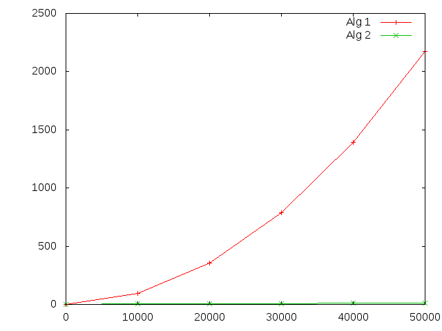
Both get slower as n increases, but algorithm 1 gets worse faster. Why does algorithm 1 suck?
What happens if we run one of them on a different computer? Will we get the same times? Probably not– processor speed, operating system, memory, and a host of other things impact how much time it takes to execute a task.
What we need, then, is a machine- and scenario-independent way to describe how much work it takes to run an algorithm. One thing that doesn't change from computer to computer is the number of basic steps in the algorithm (this is a big handwave, but generally true), so lets measure steps.
We are going to vaguely describe a "step" as a primitive operation, such as:
- assignment
- method calls
- arithmetic operation
- comparison
- array index
- dereferencing a pointer
- returning
It is important to note that this has a great degree of flexibility: one person's basic step is another person's multiple steps. To an electrical engineer, taking the not of a boolean is one step because it involves one bit. Adding two 32-bit numbers is 32 (or more!) steps. We won't be quite so anal.
So, when we determine how long an algorithm takes, we count the number
of steps. More steps = more work = slower algorithm, regardless of
the machine.
What does the following code do, and how many steps does it take?
max = a[0];                //2 steps: array index and assignment
i = 1;                     // 1 step: assignment
while (i < n)              // n comparisons, plus (n-1) times through the loop
   if (a[i] > max)         // 2: array and comparison
      max = a[i];          //2, but it doesn't always happen!
   i++;                    // 2: i=i+1;
return max;                // 1: we'll count calls and returns as 1.
This gives us: \(2 + 1 + n + (n - 1)\cdot(4 \text{ or } 6) + 1\).
Now, we're not quite done. In the code above, there are circumstances under which it will run faster than others. For example, if the array is in descending order, the code within the if statement is never run at all. If it is in ascending order, it will be run every time through the loop. We call these "best case" and "worst case" run times. We can also consider and talk about the "average" run time.
The best case is usually way too optimistic (most algorithms have best case times that are far away from average). Average case is often hard, because we need probabilistic analysis. In many cases, a worst case *bound*> is a good estimate. That way we can always say, "no matter what, this program will take no more than this many steps." In the formula above, this means the \((4\text{ or }6)\) part just becomes 6.
1.3 Comparing algorithms with bounds
In the program above, the number of steps it takes depends on the size
of the array, the n. What we really want is a function that takes
the size of the array as input, and returns the number of steps as the
output. Note that is what we developed above.
So when we're comparing algorithms, we don't compare numbers, but functions. But how do we compare functions? Which function below is "bigger"?
Well, sometimes one, and sometimes the other. So what we'll do is talk about one function dominating the other. We'll say that one function dominates another if it is always bigger than the other for every x value (for example \(f(x) = x^2\) dominates \(f(x)=-x^2\)). Neither of the functions in the graph above dominates the other.
One function can dominate another in a particular range as well. \(f(x)=1\) dominates \(f(x) = x^2\) in the range \([0;1]\).
Now, when input sizes are small, everything is fast. Differences in run time are most relevant when there is a lot of data to process. So, we colloquially ask "When n is large, does one dominate the other?" Mathematically, we ask if there exists an \(n_0\geq 1\) such that for all \(n\ge n_0\), \(f(n) \gt g(n)\) (or \(g(n) \gt f(n)\)).
In this graph, \(f(x)=3x^2-8\) dominates \(f(x)=x^2\) everywhere to the right of \(x=2\). So \(n_0=2\) - I like to call this the "crossover point".
1.4 How can we tell if one will dominate the other for large n?
It turns out it's really easy. It is all about growth rate. Take a look at this graph of \(f(n)= n^2\) vs. \(g(n) = 3n+4\).
What happens if we change the constants in \(g(n)\)? The line moves, but it doesn't change shape, so there's always some point at which f(n) passes it. Here for example is \(f(n)= n^2\) vs. \(g(n) = 30n+40\).
As soon as we start caring about really big n, it doesn't matter what the constant coefficients are, \(f(x)\) will always find a point at which it will dominate \(g(x)\) everywhere to the right. In the following table, \(f(n)\) will dominate \(g(n)\) for some large enough \(n\):
| \(f(n)\) | \(g(n)\) |
|---|---|
| \(n^2\) | \(n\) |
| \(n^2-n\) | \(5n\) |
| \(\frac{1}{10^{10}}n^2-10^{10}n-10^{30}\) | \(10^{10} n + 10^{300}\) |
1.5 Big-O
We talk about the runtime of algorithms by categorizing them into sets of functions, based entirely on their largest growth rate.
The mathematical definition: if two functions \(f(n)\) and \(f'(n)\) are both eventually dominated by the same function \(c\cdot g(n)\), where \(c\) is any positive coefficient, then \(f(n)\) and \(f'(n)\) are both in the same set. We call this set \(O(g(n))\) (pronounced "Big-Oh of \(g(n)\)"). Then we can write \(f(n) \in O(g(n))\) and \((f'(n) \in O(g(n))\).
Since the constant coefficients don't matter we say that \(g(n)\) eventually dominates \(f(n)\) if there is ANY constant we can multiply by \(g(n)\) so that it eventually dominates \(f(n)\). \(f(n)=5n+3\) is obviously \(O(n^2)\). It is also \(O(n)\), since \(f(n)\) is dominated by \(10n\), and 10 is a constant.
The formal definition: For a function \(f(n)\), if there exists a \(c\) and \(n_0\) such that \(c \gt 0\) and \(n_0 \geq 1\), and for all \(n \ge n_0, f(n) \leq c \cdot g(n)\), then \(f(n) \in O(g(n))\).
While \(f(n)=5n+10 \in O(n^2)\), it is also \(O(5n)\). \(O(5n)\) is preferred over \(O(n^2)\) because it is closer to \(f(n)\). \(f(n)\) is ALSO \(\in O(n)\). \((O(n)\) is preferred over \(O(5n)\) because the constant coefficients don't matter, so we leave them off.
2 Big-O Applications
2.1 Now we know Big-O
We're a week in, and you've already learned the most important part of this class: Big-O notation. You absolutely have to understand this to be a computer scientist. Here are some examples of Big-O notation appearing in academic papers by your faculty:
"Since the program doubles at each step, the size of \(\Psi_n\) is \(O(2^n)\)." – Chris Brown and James Davenport, "The Complexity of Quantifier Elimination and Cylindrical Algebraic Decomposition."
"The initialization in Steps 2–5 and the additions in Steps 10 and 12 all have cost bounded by \(O(n/r)\), and hence do not dominate the complexity."
– Dan Roche, "Chunky and Equal-Spaced Polynomial Multiplication"
"Unfortunately, the expressiveness of the model must be weighed against the \(O(n^3)\) cost of inverting the kernel matrix."
– Gavin Taylor, "Feature Selection for Value Function Approximation."
"Fortunately, efficient dynamic programming techniques exist to solve this exactly in \(O(k^2)\) time."
– Adam Aviv, "Practicality of Accelerometer Side Channels on Smartphones"
"Our P-Ring router, called Hierarchical Ring (HR), is highly fault tolerant, and a rounder of order \(d\) provides guaranteed \(O(log_d P + m)\) range search performance in a stable system with P peers, where m is the number of peers with items in the query range."
– Adina Crainiceanu, et al., "Load Balancing and Range Queries in P2P Systems Using P-Ring."
2.2 Comparing Two Algorithms with Big-O
We now have the language and a basic understanding of how to compare two algorithms, let's put it to the test. Suppose we have two sorted arrays of integers, and we need to determine if an integer is in the array. Consider the two search routines over that sorted array.
int find1(int A[], int toFind){

    for(int i=0;i<A.length;i++){
        if(A[i] == toFind) return i;
    }
    return -1;
}

int find2(int A[], int toFind){
    int left = 0;
    int right = A.length-1;

    while(true){
        if(right-left <= 1){
            if(toFind == A[right] && right > 0) return right;
            else if(toFind == A[left]) return left;
            else break; //didn't find it
        }

        int mid = (left + right)/2;
        if(toFind < A[mid]) right = mid-1;
        else if(toFind > A[mid]) left = mid+1;
        else return mid; // must be equal, so it's found

    }

    return -1;
}
The question is, which is faster? You might say that find(1)
should be faster because it has less code. Or, you might say, we can
only know if we run the routines, but we now know a better way with
big-O.
The first thing we need to recognize is that we are concerned with the worst-case performance, which is what Big-O measures. If we find the items in the array, we can do so really quickly. For example, it could be the first thing we look at. So the worst case performance is when we can't find the item in the array, and thus have to search the most amount for it.
In the worst case analysis, at least for find1(), let's be verbose
at first to identify the total number of steps involved. The would be:
- Initialize the variable
i, one step - Loop for
A.lengthtimes:- Compare
i<A, one step - Access
A[i], one step - Compare
A[i]andtoFind, one step
- Compare
- A return (one step) either in the loop or outside
If we say the length of the array is n, then we have 1+3n+1 total
steps, and since we don't care about constants, thats \(O(n)\). You may
notice that the driving force in the anlaysis is the total number of
comparisons that need to be performed. When we say \(O(n)\) for the find
routine, we are really saying it may take at most n comparisons to
find what is being searched for.
Turning to find2(), let's now reason about the total
number of comparisons this routine makes. The procedure is different
here because instead of searching from front to back we are leveraging
the fact that the array is sorted and making our first comparison in
the middle. In the worst case, we don't find it, so we then ask: Is
the item be searched for greater or less than what was just checked?
If it is greater, we then search in the middle of the right half, and
if it is less than, we search in the middle of the left half. This
repeats until there are only 1 or 2 items left to check.
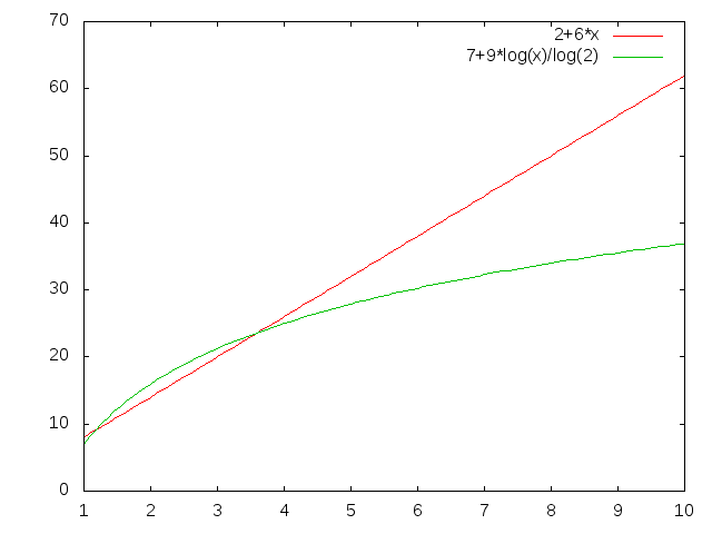
How many comparisons is that? Well, let's think of it this way, the range of items we are checking in the middle of is decreasing by a factor of 2 each time. As an example, if we have 100 items, we check once in the middle, then in the middle of 50 items, then in the middle of 25 items, then in the middle of 12 items (with rounding), then in the middle of 6 items, then in the middle of 3 items, then in the middle of 1 items. The total number of comparisons is the same as the total number of times we can divide 100 by 2 because we make one comparison per dividing the list in half.
Generalizing the problem a bit, if we have \(n\) items in the array, the total number of comparisons is the same as the number of times 2 divides into \(n\). Put another way, that is the same as solving the following for \(x\) in the following formula:
\begin{equation*} {2}^x \ge n\\ \end{equation*}Or, \(x\) is the number of times we can multiple 2 together until we get over \(n\). To solve for \(x\), we can take the \(log_2\) of both sides to get:
\[ log_2(2^x) \ge log_2(n)\\ x \ge log_2(n)\\ \]
The total number of comparisons requires is at least \(O(log_2(n))\)
which is the same as \(O(log(n)/log(2))\). Considering that \(1/log(2)\) is
a constant, we can remove that and we are left with \(O(log(n))\) as
the worst case performance of find2(). For reference, another name
for this routine is binary search and it will come up again later in
the notes.
With all of that anlaysis done, we have find1() is \(O(n)\) and
find2() is \(O(log(n))\), so we can now say that find2() should be
faster, and it is!
2.3 Our Main Big-O Buckets and Terminology
As we just saw, big-O is extremely useful because it allows us to put algorithms into buckets, where everything in that bucket requires about the same amount of work. It also allows us to arrange these buckets in terms of performance.
First, though, it's important that we use the correct terminology for these buckets, so we know what we're talking about. In increasing order…
- Constant time: The run time of these algorithms does not depend on the input size at all. \(O(1)\).
- Logarithmic time: \(O(\log(n))\). Remember, changing the base of the log is exactly the same as multiplying by a coefficient, so we don't tend to care too much if it's natural logarithm, base-2 logarithm, base-10 logarithm, or whatever.
- Linear time: \(O(n)\).
- n-log-n time: \(O(n \log(n))\).
- Quadratic time: \(O(n^2)\).
- Cubic time: \(O(n^3)\).
- Polynomial time: \(O(n^k)\), for some constant \(k\gt 0\).
- Exponential time: \(O(b^n)\), for some constant \(b \gt 1\). Note this is different than polynomial.
Fuzzily speaking, things that are polynomial time or faster, are called "fast," while things that are exponential, are "slow." There is a class of problems that are believed to be slow called the NP-complete problems. If you succeed in either (a) finding a fast algorithm to compute an NP-complete problem, or (b) prove that no such algorithm exists, congratulations! You've just solved a Millenium Problem get a million dollars, and are super-famous. If you take the algorithms class, you'll learn how to do that.
The following table compares each of these buckets with each other, for increasing values of \(n\).
| \(n\) | \(\log(n)\) | \(n\) | \(n\log(n)\) | \(n^2\) | \(n^3\) | \(2^n\) |
|---|---|---|---|---|---|---|
| 4 | 2 | 4 | 8 | 16 | 64 | 16 |
| 8 | 3 | 8 | 24 | 64 | 512 | 256 |
| 16 | 4 | 16 | 64 | 256 | 4096 | 65536 |
| 32 | 5 | 32 | 160 | 1024 | 32768 | 4294967296 |
| 64 | 6 | 64 | 384 | 4096 | 262144 | 18446744073709551616 |
| 128 | 7 | 128 | 896 | 16384 | 2097152 | 340282366920938463463374607431768211456 |
| 256 | 8 | 256 | 2048 | 65536 | 16777216 | 115792089237316195423570985008687907853269984665640564039457584007913129639936 |
| 512 | 9 | 512 | 4608 | 262144 | 134217728 | 13407807929942597099574024998205846127479365820592393377723561443721764030073546976801874298166903427690031858186486050853753882811946569946433649006084096 |
| 1024 | 10 | 1024 | 10240 | 1048576 | 1073741824 | 179769313486231590772930519078902473361797697894230657273430081157732675805500963132708477322407536021120113879871393357658789768814416622492847430639474124377767893424865485276302219601246094119453082952085005768838150682342462881473913110540827237163350510684586298239947245938479716304835356329624224137216 |
To understand just how painful exponential time algorithms are, note that the number of seconds in the age of the universe has about 18 digits, and the number of atoms in the universe is a number with about 81 digits. That last number in the table has 309 digits. If we could somehow turn every atom in the universe into a little computer, and run all those computers in parallel from the beginning of time, an algorithm that takes \(2^n\) steps would still not complete a problem of size \(n=500\).
2.4 Other Big-Stuff
Through this entire section, we are still talking about worst-case run times.
Remember, if \(f(n)\in O(g(n))\), then we can come up with a \(c\) such that for all \(n \ge n_0\), \(f(n)\leq c\cdot g(n)\).
If we replace the second part of that definition with a greater-than like \(f(n) \ge c \cdot g(n)\), then \(f(n)\in \Omega (g(n))\). That is read, "big-Omega" of \(g(n)\) and we can think of this as a lower bound, meaning, for an algorithm, it can't essentially be faster than the \(g(n)\).
Generally, we use Big-Omega when describing the best case performance of an algorithm because we are concerned with the lower-bound on how fast a routine can complete. When we are performing a worst case analysis, we are concerned with bounding how slow a routine can complete, and thus we use Big-O.
As an example of \(\Omega\) analysis, return to the two find routines
above. In that analysis, we said the worst case is \(O(n)\) for
find1() and \(O(log(n))\) for find2(), but what about the best case
analysis? As identified, we could find the searched item on our first
comparison, so both routines are \(\Omega(1)\), or constant time best
case.
Sometimes, when performing an analysis you'll find that the Big-O upper-bound and the Big-Omega lower-bound are the same. When this happens, we call this Big-Theta, and it is a special case where \(f(n)\in O(g(n))\), and \(f(n)\in\Omega(g(n))\). Obviously, big-Θ is most precise "Big" notation. In this class, we'll mostly talk big-O. If you take algorithms, that will mostly be big-Θ.
2.5 Analyzing Selection Sort
Let's consider one more routine for analysis, say selection sort, something you should remember from your intro to computing class.
void selectionSort(int A[]){
    for(int i=0;i<A.length-1;i++)
        for(int j=i+1,j<A.length;j++)
            if(A[i] > A[j])
                swap(A,i,j); //swap routine
}
Starting with the worst-case analysis, using our big-O analysis tools, we need to identify the dominate step, which in this case is going to be how many comparisons must be made to ensure that all the right elements are swapped to get a sorted ordering. To make the math easier, without generalization, lets say that the array has \(n+1\) elements in it. Then the number of comparisons we must make
\[ \sum^{n}_{i=0} n-i \]
That is, the first time through the inner loop, we do n comparison, then n-1, then n-2, and so on until we do 2, and then finally 1. If we reverse the order, of the summation, say add 1, 2, …, n-1, n, then we can write the summation more simply like so:
\[ \sum^{n}_{i=1} i = \frac{n(n+1)}{2} \]
The solution to the sum of the numbers between 1 and n is known to be the common formula, \(n(n+1)/2)\). To quickly give you the intuition why this is so, consider doubling the items in the summation and then reversing the order of one series of sums and aligning the two series such that the first and the last number in each summation series align. Visually, you'd get something that looked like this:
\begin{array} \quad & 1 &+& 2 &+& 3 &+& \ldots &+& n-2 &+& n-1 &+& n\\ + & n &+& n-1 &+& n-2 &+& \ldots &+& 3 &+& 2 &+& 1\\ \hline \quad & n+1 &+& n+1 &+& n+1 &+& \ldots &+& n+1 &+& n+1 &+& n+1 \quad = \quad n(n+1)\\ \end{array}And since we doubled the list, dividing by 2 gives the desired result of \(n(n+1)/2\) or \(1/2(n^2+n)\). As the \(n^2\) dominates, selection sort is \(O(n^2)\)
Let's consider now a best case analysis of selection sort. How fast could selection sort possibly run? It turns out that it is \(\Omega(n^2)\). No matter the input length \(n\), it will take at least \(\Omega(n^2)\) comparison steps because the routine can't be sure if it is sorted ahead of time. Thus \(n^2\) is a lower bound and an upper bound on performance for selection sort for a best-case and worst-case scenario.
As the the upper and lower bound are the same for the best-case and worst-case scenario, then we can say that in the average-case that selection sort is Θ(n2).
3 Big-O of Arrays and Linked Lists
3.1 Analyzing Data Structures we already know
We are already quite comfortable with two types of data structures: arrays, and linked lists (we also know array lists, but those require some more complicated analysis). Today we're going to apply our analysis skills to the operations we commonly do with these data structures.
3.2 Access
"Access" means getting at data stored in that data structure. For example, getting the third element.
In an array, this is really easy! theArray[3] Does the time this
takes depend upon the size of the array? No! So, it's constant time.
\(O(1)\).
In a Linked List, this is harder. Now, if we were looking for the first element, or the third element, or the hundredth element, then that does NOT depend upon the size of the list, and that would be \(O(1)\). However, remember that we are interested in worst case, and if we think about this as a game where an adversary gets to choose which element to make our algorithm the slowest, then what would he choose?
You might think that the adversary should choose the last element, but that could be O(1) because many linked list are doubly linked with a reference to the head and tail of the list and pointers between nodes pointing forward and backwards. In fact, the worst case element to reference is right in the middle, which is furtherest from the head and tail references requiring at least \(n/2\) pointer follows to be reached. Thus, access for Linked Lists is \(O(n)\).
(As an aside, you might be saying, why not just store a reference to the middle item too to remove the worst case? Then, the worst case shifts to the middle of the two halfs, requring \(n/4\) pointer follows, and we are back at \(O(n)\). Taking this one step further, you might just say, why not just store two more references to the two node in the middle of the two halves, but then the worst case shifts again to be the middle of any of the four segments leaving us with \(n/8\) and still \(O(n)\). You can keep doing this, adding references ad infinitum, but then you need to store and manage \(n\) references to each of the \(n\) nodes: what structure are you going to store them in?! Another Linked Lists an Array? And, then you're back where you started, and the logic falls a part.)
3.3 Adding an Element to the Front or Back
In an array, this is hard! Because we now have an additional element to store, we have to make our array bigger, requiring us to build a new array of size \(n+1\), move every element into it, and add the new one. That "move every element into it," will take \(O(n)\) time.
In a linked list, this is really easy! If we have a pointer to the first and last link in the chain, this takes the same amount of time, no matter how long the list is! \(O(1)\).
It's worth noting that removing an element requires a similar process.
3.4 Adding an Element to a Sorted List or Array
The scenario: assume the array or list is in sorted order, and we have a new element to add. How long will it take (as always, in the worst case)?
This is a two-step process: (1) find where the element goes, and (2) add the element.
In arrays, we recently saw two ways to do (1); one where we cycled through the entire array looking for the proper location (\(O(n)\), and one where we repeatedly halved the array until we found the spot (this is called binary search, and takes \(O(log(n))\)). Doing step (2) is very similar to what we had to do for adding an element to the front or back, so that step is \(O(n)\). So, in total, this takes us \(O(log(n)) + O(n)\), which is \(O(n)\).
Alternatively, you could skip binary search, and do a sequential search (go from element to element, front to back until you find it), moving elements to the new array as you go. Once you find the location to add your new element, add it to the new array, and continue moving elements. This gives you two loops, each of which move roughly half the array. Again, in total, this gives us \(O(n)\).
In a linked list, doing step (1) is \(O(n)\) (see why?). Adding the element at that point is \(O(1)\). So, in total, \(O(n)\).
In summary, it's \(O(n)\) for either an array or a linked list. But there's a big difference in how this breaks down. For arrays, the \(O(n)\) really comes from the "insertion" part, whereas for linked list the insertion part is easy and the \(O(n)\) comes from the "search" part. This difference will come into play in some applications later on.
3.5 Traversal
Traversal is our word for "visiting every element." It should be clear that for both arrays and linked lists, this is \(O(n)\).
3.6 Why did we do this?
The executive summary is as follows:
| Array | Linked List | |
|---|---|---|
| Access | \(O(1)\) | \(O(n)\) |
| Insertion/Remove from front/back | \(O(n)\) | \(O(1)\) |
| Sorted insertion/remove | \(O(n)\) | \(O(n)\) |
| Traversal | \(O(n)\) | \(O(n)\) |
We'll be doing this all semester, for each of our data structures. As you can see, the choice between arrays and linked lists, comes down to what you're doing with them. Doing lots of access? Use an array. Adding and removing elements often? Use a linked list. This give-and-take is at the center of Data Structures.
Credit: Ric Crabbe, Gavin Taylor and Dan Roche for the original versions of these notes.